American Automobility: An Exploration Into the Factors Which Influence the Choice to Forgo Car Ownership in the New York Metropolitan Area
MAY 14, 2022
Examining the New York Metropolitan Area, this paper explores which factors influence the percentage of households that opt to forgo car ownership. This paper uses a linear regression model to conclude that, while wealth is not correlated with the percentage of zero-car households in a given county, the amount of suitable substitutes for driving (such as walkability and robust public transit) and population density are correlated with the percentage of zero-car households. This is my final paper for my spring 2023 econometrics class.
Introduction
The automobile has traditionally been the cornerstone of the American Dream. Beginning with the popularity and affordability of the Ford Model T in the early 1900s, cars have been ingrained in American life for over a century. To this day, the car industry in the United States is large and continuously growing. Over 280 million cars are registered in America. The yearly revenue of the American automobile industry peaked in 2021, exceeding $1.5 trillion. Over 5.4 cars are sold in the United States every minute. Of the new cars sold, the overwhelming majority are light trucks (such as vans, minivans, or pickup trucks) as opposed to sedans or heavy trucks. In 1949, only 3% of American families owned more than one car. By 2022, that number had risen to 59.1%. Over 3.1 trillion miles were driven on American roads in 2022.
Despite automobiles’ prominence in the United States, concerns over automobility and car-dependency have grown in recent years due to the negative economic, environmental, and social impacts of car ownership. There are five primary negative consequences of automobiles. First, cars shackle Americans to debt. Earlier in 2023, the average new car price rose to an all-time high of $50,000. The average monthly cost of car ownership (including gas, maintenance, and the car itself) is $716 per month. These costs result in automobile debt being the third largest type of American debt. Exceeding $1.5 trillion, American car debt is larger than credit card debt (but smaller than student loan debt and mortgages). The American government’s construction of car-dependent infrastructure also poses a significant financial burden to citizens, even if those citizens do not own a car. In 2018, for instance, federal, state, and local governments spent a combined total of over $186.1 billion on highway and road expenditures.
Second, car-dependency poses a serious safety threat. Between 35,000 and 46,000 Americans die from road traffic fatalities every year. Over 4 million additional people annually are injured in car crashes seriously enough to require medical attention. In total, car crashes have killed over 3.2 million Americans to date. By comparison, more Americans have died in car fatalities than every war Americans have fought in combined. There’s a 0.5% chance that our lives will end in a car crash and a 33% chance we will eventually be seriously injured in one. Moreover, automobile fatalities are a uniquely American problem. While the United States has 14.5 traffic fatalities per 100,000 people, Germany has 7.1, Japan has 5.8, and the United Kingdom has 5.3.
Third, automobiles are one of the biggest contributors to anthropogenic climate change. Transportation is America’s largest-emitting sector, ahead of electric power, industry, housing, and agriculture. Transportation in America emits over 1.8 billion metric tons of greenhouse gasses. Americans consume 1/4th of the world’s oil, or 850 million gallons of crude oil per day (2.8 gallons per person per day). Importantly, light trucks (America’s highest selling category of car) are not subject to the fuel efficiency laws typical cars must abide by and, as such, emit significantly more carbon dioxide. If the total 2018 carbon emissions of SUV drivers were compared to nations, they would be ranked seventh for carbon emissions.
Fourth, the parking required by cars is a blight on cities. Parking covers more acres of American cities than any other singular thing. Surface parking lots alone cover 5% of urban American land, a size bigger than Rhode Island and Delaware combined. The cost of all of America’s parking spaces exceeds the value of all cars. In fact, the cost of all American parking is around the cost of all American cars and all American roads combined. Despite the enormous cost, many parking spots spend the majority of their life not being used. A nationwide count in 2010 found that there are over 500 million empty parking spaces in America at any given time.
Fifth, car-dependent urban form exacerbates racial inequality. Over 200,000 Americans — largely Black and Hispanic — have lost their homes to federal highway projects via eminent domain over the last thirty years.
Given these negative impacts, it might be beneficial for some Americans to forgo car ownership. To that end, this paper aims to answer which factors determine whether or not households own automobiles.
I will narrow this paper’s focus to the New York metropolitan area. The largest and one of the most populous metropolitan areas in the world, the New York metropolitan area includes New York’s five burrows, Long Island, and many nearby New York, New Jersey, and Connecticut cities (such as Newark, Jersey City, Bridgeport, and New Haven). I chose to focus on the New York metropolitan area because of the region’s vast diversity in land use; the New York metropolitan area includes dense skyscrapers with mixed-use zoning and multi-family housing (in Manhattan, Brooklyn, and Jersey City), suburban areas with detached, single-family homes (in Paterson, Stamford, and Long Island), and more rural areas with low population density (in parts of New Jersey, Connecticut, and Upstate New York). Given that I’m interested in how the design of American cities can impact car ownership rates, the diversity of land use will make the area a good sample.
Review of Existing Literature
International
London. The Roads Task Force of Transport for London — the department of London’s government responsible for the city’s transport network — published a thematic analysis in 2012 entitled “How many cars are there in London and who owns them?” The analysis concludes, “Londoners are more likely to own a car if they live in outer London, live in an area with poor access to public transport, have a higher income, have a child in the house, and are of Western European nationality.”
The Netherlands. Researchers at the Amsterdam Institute for Social Science Research used logistic regression analysis in a 2016 paper entitled “Determinants of car ownership among young households in the Netherlands: the role of urbanization and demographic and economic characteristics.” The authors conclude that urbanization level (defined on a scale abstracted from number of addresses per square kilometers in the four‐digit postcode area of a household's address) and household composition (categorized as either young singles, young couples, young two‐parent families and young single‐parent families) are two essentials factors determining car ownership in the Netherlands. Furthermore, the study “Household Car Ownership in the Netherlands” by Delft University of Technology researcher Yannick Maltha found, “the influence of household income on car ownership has decreased considerably over time (from 38% in 1987 to 28% in 2014).”
Canada. In a 2008 study entitled “Dependence on cars in urban neighbourhoods,” researcher Martin Turcotte examined the factors influencing whether or not Canadians own cars. Working on behalf of Statistics Canada (the country’s national statistics office), Turcotte concluded that the most important factors influencing car ownership among Canadians are the physical form of the urban neighborhood they live in. The study finds, “neighbourhoods composed primarily of typically suburban dwellings and located far from the city centre were characterized by an appreciably higher level of automobile dependence.” University of British Columbia researcher Tamim Raad arrived at very similar conclusions in his 1998 study “The car in Canada: a study of factors influencing automobile dependence in Canada’s seven largest cities.” Examining Canada’s seven largest cities, Raad finds that urban density and transit supply are negatively correlated with car ownership, whereas the amount of parking supply in a city’s central business district is positively correlated with car ownership.
Domestically
Research around variables impacting car ownership rates in America dates back to 1966. In “Trends in Automobile Ownership and Indicators of Saturation,” economist for the US Bureau of Public Roads Walter Bottiny concludes that personal income per capita is strongly positively correlated with automobile ownership regardless of US state. Bottiny also finds that population density and availability of public transportation are negatively correlated with car ownership rates (especially in San Francisco and New York metropolitan areas).
These trends largely continue to hold in the twenty-first century. The American Association of State Highway and Transportation Officials’s 2021 report “Commuting in America: The National Report on Commuting Patterns and Trends,” for instance, aims to explain the recent decline in zero-car American households. Using data from the 2017 National Household Travel Survey, the report concludes population density, availability of car transportation alternatives (such as walking, biking, and transit), and the perceived financial burden of cars are all negatively correlated with household automobile ownership. Entitled “Factors Affecting Automobile Ownership and Use,” a 1992 study of Chicago suburbs likewise concluded, “Location of residence or workplace, or both, and residence relocation into outer-ring, low-density suburbs affect automobile ownership positively, whereas workplace locations in the central city affect automobile ownership negatively because of the availability of high-quality commuter rail service.”
Theoretical Model
% of Zero-Car Households = f (low wage workers (+), population density (+), walkability (+), distance to transit (-))
The response variable I’m interested in is the percentage of zero-car households. There are four explanatory variables I’m interested in. The first explanatory variable is the number of low wage workers. I expect this variable to be positively correlated with the percent of households without cars. As the number of low wage workers increases, the percentage of homes without cars (a normal good) should increase as well. The second explanatory variable is population density. I expect this variable to be positively correlated with the percent of households without cars. As population density increases, people need to travel less to access common urban amenities (and thus have less need for a car). The third explanatory variable is walkability. I expect this variable to be positively correlated with the percent of households without cars. If more parts of a city can be accessed on foot, there is less need to own a car. Finally, the fourth explanatory variable is the distance to the nearest public transit stop. I expect this variable to be negatively correlated with the percent of households without cars. As the distance to the nearest transit stop decreases, citizens have an easier time accessing public transit and less need to own a car.
Data Description
This paper will draw upon the Environmental Protection Agency’s Smart Location Database. The database includes over 110 variables “summarizing characteristics such as housing density, diversity of land use, neighborhood design, destination accessibility, transit service, employment, and demographics.” The EPA released the first version of the Smart Location Database in 2011. This paper uses the latest version of the Smart Location Database (version 3.0), released in 2021. While the Smart Location Database reports variables by the census block group, I will abstract each variable to the county level for this analysis. The Smart Location Database divides the New York Metropolitan Area into twenty-eight distinct counties.
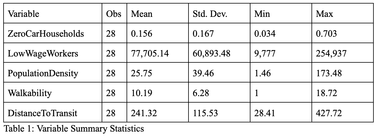
The response variable — the percentage of zero-car households in a given county — is labeled “pct_ao0” in the Smart Location Database. In this paper, I will refer to this variable as “ZeroCarHouseholds” for clarity. Table 1 displays the summary statistics of this variable. The mean percentage of households with no cars is 15.6%. With 70.3% of households opting to forgo car ownership, New York County (more commonly referred to as Manhattan) has the highest percentage of zero-car households in the sample. Manhattan is one of New York City’s five boroughs and is home to many of the landmarks most often associated with New York City (such as Central Park, the Empire State Building, and Times Square). On the other end of the spectrum, Hunterdon County, New Jersey has the lowest percentage of zero-car households at 3.4%. Hunterdon County has the third-highest personal income per capita out of all New Jersey counties and the nineteenth highest personal income per capita out of all counties in the United States.
The first explanatory variable — the number of low wage workers — is measured as the count of workers making less than $1250 per month in a given county. This variable is labeled “R_LowWageWk” in the Smart Location Database. In this paper, I will refer to the variable as “LowWageWorkers” for clarity. The mean number of low wage workers in a county is 77,705.14 people. The county with the fewest low wage workers in the sample is Putnam County, New York. Putnam County is a one-hour drive away from Midtown Manhattan and serves as a suburb of New York City. With only 9,777 low wage workers, Putnam County is one of the most affluent countries in America. The county with the most low wage workers (at 254,937 people) is Kings County, more commonly known as Brooklyn. Nearly one of five Brooklyn residents live in poverty, and more Brooklyn children live in poverty than any other New York City borough.
The second explanatory variable — population density — is measured in people per acre. This variable is labeled “D1b” in the Smart Location Database. In this paper, I will refer to the variable as “PopulationDensity” for clarity. The mean population density is 25.75 people per acre. Monroe County, New York has the lowest population density in the sample. Located in the rural Finger Lakes Region of New York State, Monroe County has 1.46 people per acre. At 173.48 people per acre, New York County (Manhattan) has the highest population density.
The third explanatory variable — walkability — is labeled as “D4A_Ranked” in the Smart Location Database. This variable is generated by the EPA. Between the values of 1 and 20, the variable ranks the walkability of a given county (with 1 being not walkable and 20 being very walkable). In this paper, I will refer to the variable as “Walkability” for clarity. The mean walkability value is 10.19. The county with the lowest walkability score is Sussex County, New Jersey. Sussex County is the northernmost county in New Jersey. With a walkability score of 1 out of 20, Sussex County is rural and largely forested. The county with the highest walkability score is New York County (Manhattan). Manhattan has a walkability score of 18.72 out of 20; Manhattan residents often accomplish many of their daily tasks by foot.
Finally, the fourth explanatory variable — distance to transit (such as bus, subway, or light rail transit) — is measured as the distance from the population-weighted centroid to nearest transit stop in meters. This variable is labeled “D4a” in the Smart Location Database. In this paper, I will refer to the variable as “DistanceToTransit” for clarity. The mean distance from the population-weighted centroid to nearest transit stop is 241.32 meters. At 28.41 meters, the county with the lowest DistanceToTransit is Ulster County, New York. Located along the Hudson River, Ulster County is around 100 miles away from Manhattan. The county is a combination of suburban development (in cities such as Kingston and New Paltz) and rural land (such as the Slide Mountain Wilderness Area, the largest state-owned forest preserve in the Catskill Mountains). Ulster County is serviced by Ulster County Area Transit, a county-owned bus operator. At 427.72 meters, the county with the highest DistanceToTransit is Nassau County, New York. Nassau County, around 30 miles away from Manhattan, is located on Long Island. Composed of affluent suburbs, Nassau County contains four of America's top ten towns by median income.
Figures 1-4 show the relationship between ZeroCarHouseholds and the four explanatory variables.
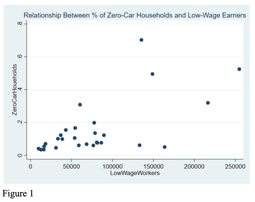
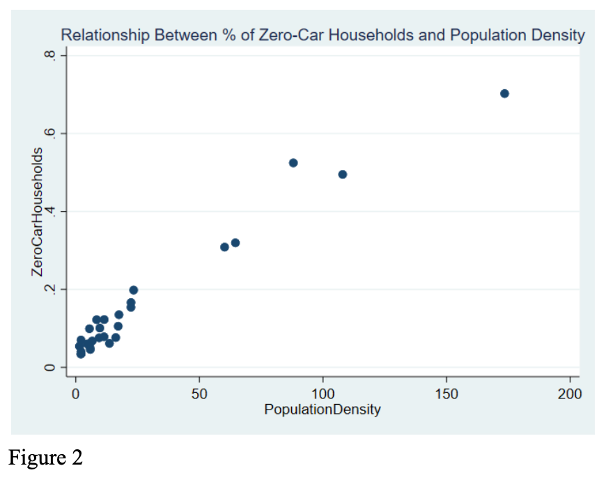
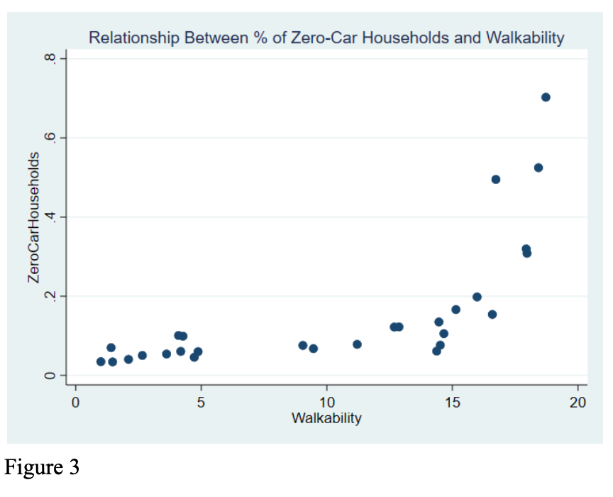
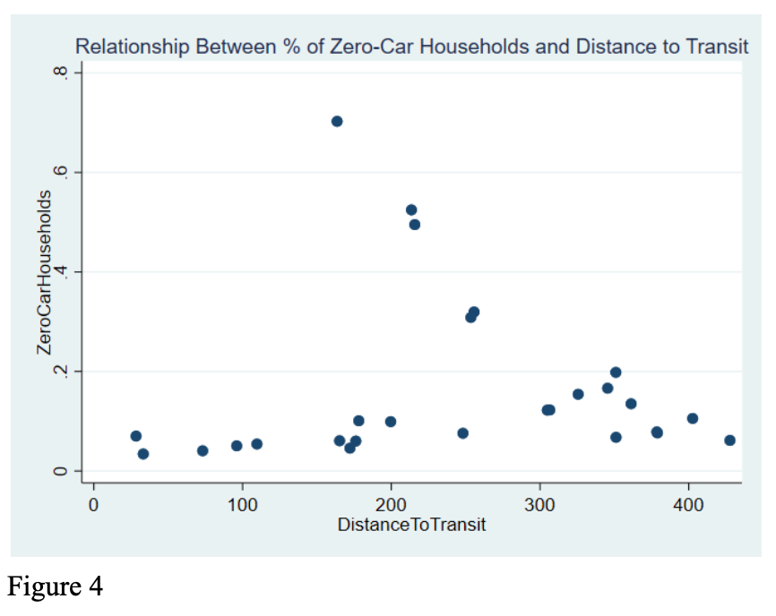
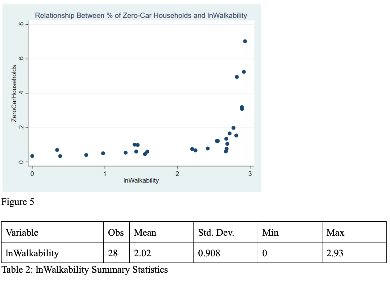
While figures 1, 2, and 4 show a linear relationship, figure 3 shows a logarithmic relationship. As such, I will take the natural log of the Walkability variable.
Because this data is cross-sectional, I decided to check for heteroscedasticity. I performed both the White test and the Breusch–Pagan test. Neither came back with evidence of heteroscedasticity:
White's general test statistic: 17.69057 Chi-sq(14) p-value = 0.2212
Breusch-Pagan LM statistic: 2.29 Chi-sq(1) p-value = 0.1306
I also wanted to see if there was a notable linear relationship between the regressors, so I decided to check for multicollinearity. There are no highly correlated variables in the correlation matrix in Table 4, so there’s no strong evidence of multicollinearity.
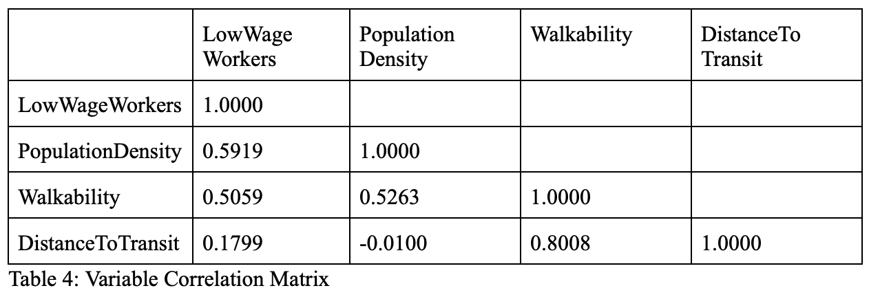
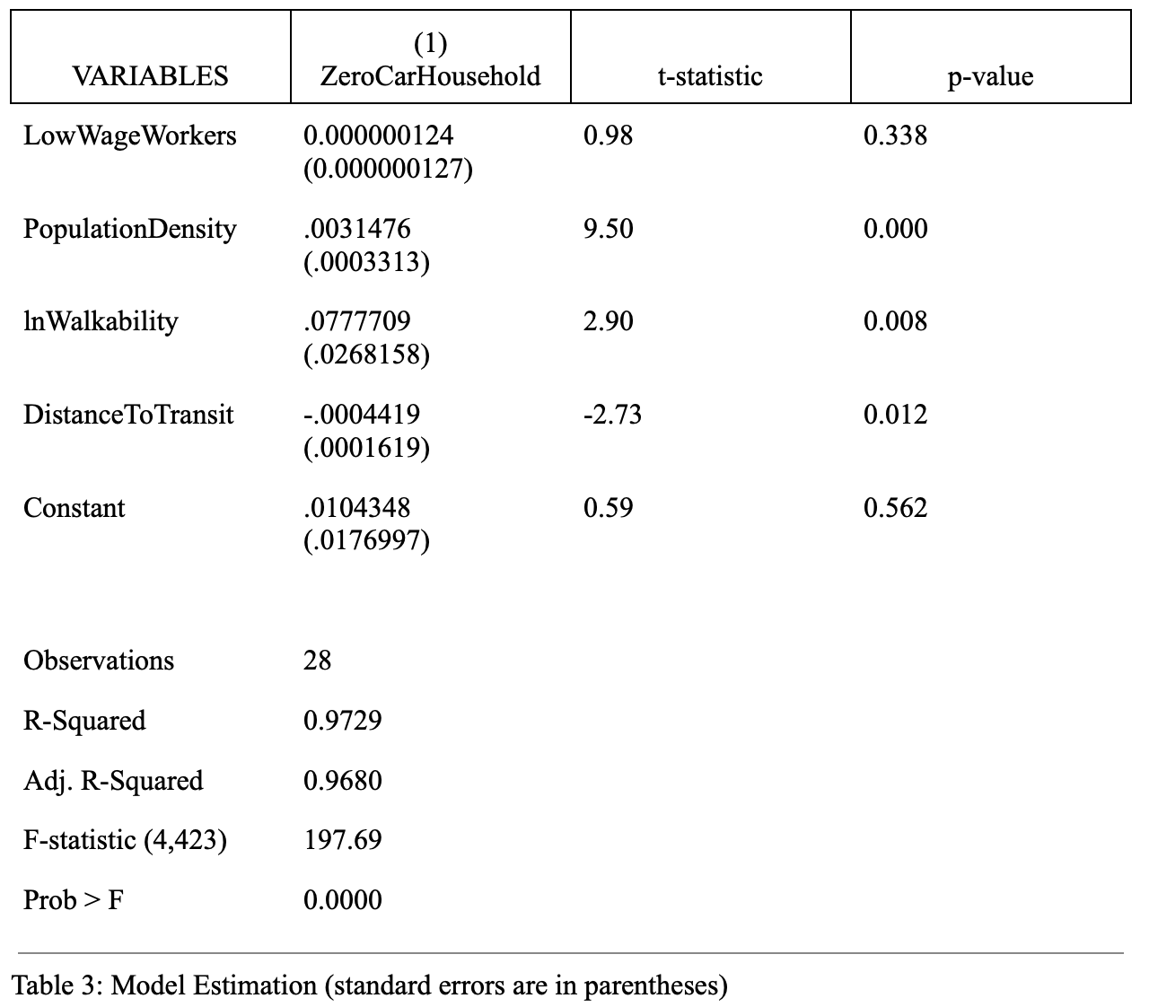
Given that I have found no evidence of heteroscedasticity or multicollinearity, I will not change my model. The final model is: ZeroCarHouseholds = 0.0104348 + 0.000000124LowWageWorkers + 0.0031476PopulationDensity + 0.0777709lnWalkability
-0.0004419DistanceToTransit + ui
-0.0004419DistanceToTransit + ui
Interpretation
The adjusted R^2 of this model is 0.9680, which is very high. This value means that 96.80% of the variation in the percentage of zero-car households can be explained through the four included explanatory variables. The y-intercept of this model resists economic interpretation, as there is no county with the PopulationDensity, DistanceToTransit, or LowWageWorkers variables equal to 0.
When the number of low wage workers in a county increases by 1, the percentage of zero-car households increases on average by 0.000000124. This positive relationship agrees with my a priori assumption; cars are very expensive, so a region with many low wage workers would be less able to afford cars. Interestingly, this coefficient is not significant at α=0.05; the t-statistic is 0.98 and the p-value is 0.338. This high p-value signifies that we can not conclusively reject the hypothesis that this explanatory variable has an impact on the response variable. In other words, we cannot confidently say that wealth impacts car ownership rates. This finding was unexpected; I initially thought wealth would impact car ownership rates.
For a 1 person per acre increase in population density, the percentage of zero-car households increases on average by 0.0031476. This coefficient is significant at α=0.05, as the t-statistic is 9.50 and the p-value is 0. This positive relationship agrees with my a priori assumption; when people have more of the city amenities they need in a smaller space, people have less need for a car.
For a 1 unit increase in the natural log of Walkability, the percentage of zero-car households increases on average by 0.0777709. This coefficient is significant at α=0.05, as the t-statistic is 2.90 and the p-value is 0.008. This positive relationship agrees with my a priori assumption; walking is a substitute for driving. When people can access more on foot, they have less need for a car.
For a 1 meter increase in the distance from the population-weighted centroid to nearest transit stop in meters, the percentage of zero-car households decreases on average by 0.0004419. This coefficient is significant at α=0.05, as the t-statistic is -2.73 and the p-value is 0.012. This negative relationship agrees with my a priori assumption; when people can access public transit more easily, people have less need to own cars.
Concluding Remarks
In future research, I’m interested in seeing if the trends I identified hold for other metropolitan areas in America. The New York Metropolitan Area is rather unique in the American context as it has better public transit, more walkability, and greater urban density than nearly every other American metropolitan area. Would the trends espoused in this linear regression model hold for the San Francisco Metropolitan Area or the Chicago Metropolitan Area?
If I were to go about re-estimating my model, I’d like to incorporate other variables not present in the EPA’s Smart Location Database. For example, University of Leeds researchers (focusing primarily on America but also incorporating data from over 25 other countries) researched the impact on gasoline prices (a complement to cars) on car ownership rates. Publishing their findings in a paper entitled “Elasticities of Road Traffic and Fuel Consumption with Respect to Price and Income: A Review,” researchers reviewed 69 empirical studies published since 1990 and found that a 10% increase in the real price of gasoline is correlated with a 1% reduction in vehicle miles traveled and a less than 1% decrease on net vehicle ownership.
The findings in this paper present important policy implications for urban design. If American citizens want to discourage car ownership, a reliable way to achieve this goal is to provide robust substitutes (such as walkability, urban density, and transit access) to driving. This paper will conclude by presenting two feasible policy proposals which will improve these substitutes.
Remove off-street parking minimums. Off-street parking minimums set by city governments are often chosen arbitrarily. For example, University of California, Berkeley researchers surveyed 49 San Francisco Bay Area cities in 1997 and found that each city had drastically different minimum parking requirements for hospitals of the same capacity. When the researchers asked city officials in charge of setting parking minimums how they came up with those numbers, 70% said they did not know or guessed.
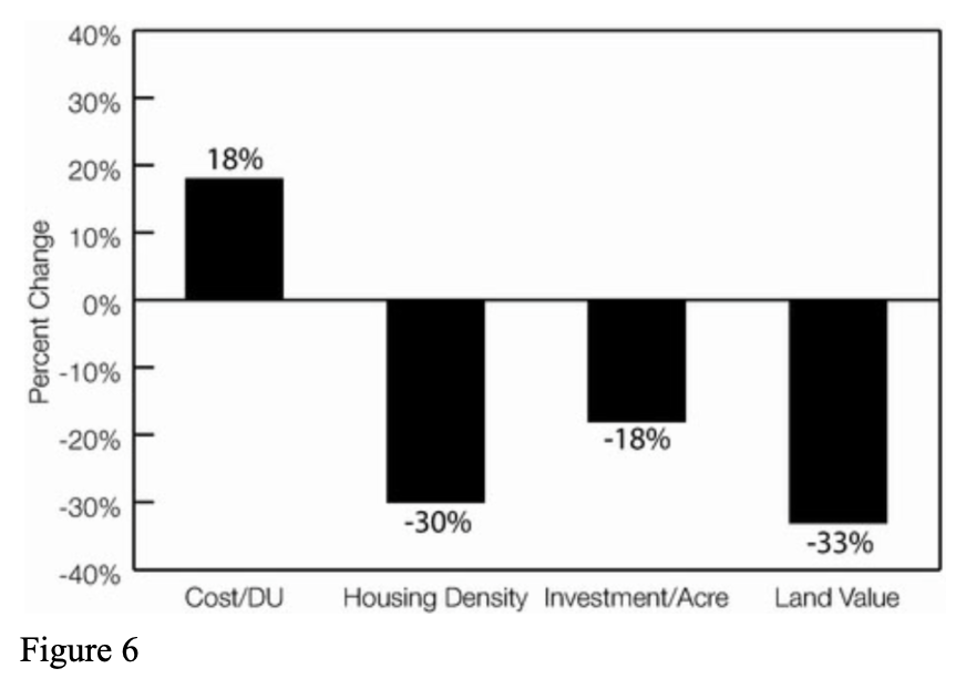
A parking space occupies an average of 300 square feet, and this large spatial footprint reduces walkability. Additionally, mandatory off-street parking minimums for housing units increases the cost of housing and decreases population density. In 1964, University of California, Berkeley economist Brian Bertha researched the impact of Oakland’s 1961 requirement of one parking space per housing unit. After examining data from 45 Oakland apartment buildings developed in the four years before the parking mandate and 19 apartment buildings developed in the two years after, Bertha concluded that the parking minimum increased the construction cost per apartment by 18% and reduced housing density by 30%. Figure 6 shows the impact of this legislation on housing cost, housing density, housing investment, and land value.
Similarly, University of California, Berkeley economists Wenyu Jia and Martin Wachs found in 1998 that San Francisco’s requirement of one parking space per housing unit adds an additional 20% to the cost of affordable housing. The researchers conclude that eliminating this requirement would allow 24% more San Franciscans to buy homes.
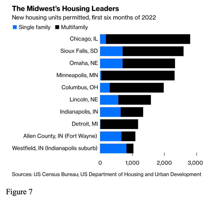
Eliminate single-family zoning. Single-family zoning is a residential code which restricts the number of units developers can build on a single plot of land. Minneapolis, Minnesota can serve as a case study of how eliminating single-family zoning can impact a city. Before the Minneapolis City Council eliminated single-family zoning city-wide in 2018, around 70% of the city’s land was zoned for detached single-family houses. Four years later, Minneapolis permitted nearly as many multifamily units (2,285) as Chicago (2,628), a city over five times Minneapolis’s size.
On top of increasing population density, eliminating single-family zoning also leads to increases in walkability (as residents are able to access more of the city within a shorter distance) and the distance from the population-weighted centroid to public transit (as more residents are clustered in denser urban cores closer to transit stops).
These two policies and others which increase walkability, population density, and transit access provide viable alternatives to automobile ownership and car-dependent urban form.
References for this paper can be found here.